Glycemic control | Theory of Hybrid Systems

Classification

# of variables	# of modes	# of jumps
4	2-3	1-4

Type	Continuous dynamics	Guards & Invariants	Resets
hybrid	non-polynomial	linear polynomial	identity

Download

Flow* Strategy I	glucose_control_I
Flow* Strategy II	glucose_control_II
Flow* Strategy III	glucose_control_III

Model description

We study the “minimal model” defined in [1-3] for the dynamics of glucose and insulin interaction in the blood system. It is described by the following ODE.

$\left\{ \begin{array}{lcl} \dot{G} & = & -p_1 \cdot G - X\cdot(G + G_B) + P \\ \dot{X} & = & -p_2\cdot X + p_3\cdot I \\ \dot{I} & = & -n\cdot (I + I_B) + \frac{u}{V_I} \end{array} \right.$

wherein $p_1,p_2,p_3$ are constant parameters whose typical values are $p_1 = 0$ min $^{-1}$ , $p_2 = 0.025$ min $^{-1}$ and $p_3 = 0.013$ min $^{-2}$ U $^{-1}$ L. The values of $G_B$ and $I_B$ are the basal values of plasma glucose concentration and free plasma insulin concentration respectively, and they are given by $G_B = 4.5$ mmol L $^{-1}$ , $I_B = 0.015$ U L $^{-1}$ . The constant $V_I$ is the insulin distribution volume, and the value of $n$ denotes the fractional disappearance rate of insulin. We take their values as $V_I = 12$ L and $n = \frac{5}{54}$ min $^{-1}$ . The remaining parameters are variables, we give their explanations as below.

$G$	the difference of plasma glucose concentration
$I$	the free plasma insulin concentration
$X$	the insulin concentration in an interstitial chamber
$P$	the rate of infusion of exogeneous glucose
$u$	the rate of infusion of exogeneous insulin

We use the formulation $P = 0.5 \cdot \exp(-0.05\cdot t)$ given in [4] for the rate of insulin infusion, and consider three different strategies for the insulin delivery rate $u$ .

Strategy I is proposed in [5].
The rate $u$ is $0.5$ U h $^{-1}$ when $G < 4$ mmol L $^{-1}$ ,
and it is $2.5$ U h $^{-1}$ when $G > 8$ mmol L $^{-1}$ .
If $G$ is in the range from $4$ to $8$ mmol L $^{-1}$ , we use $u = (0.5\cdot G - 1.5)$ U h $^{-1}$ which is a linear transition between the rates $4$ and $8$ mmol L $^{-1}$ .

Strategy II is taken from [6], it is similar to Strategy I but considers the rates $2$ and $12$ mmol L $^{-1}$ .
That is, we set $u = 0.5$ U h $^{-1}$ when $G < 2$ mmol L $^{-1}$ ,
and $u = 2.5$ U h $^{-1}$ when $G > 12$ mmol L $^{-1}$ .
For the case that $G$ is between $2$ and $12$ mmol L $^{-1}$ , $u$ is defined by $(0.2\cdot G + 0.1)$ U h$^{-1}$ .

In order to better stabilize the glucose level, a more sophisticated control strategy is presented in [6]. We call it Strategy III. The controller reads the value of $G$ in the beginning of every $3$ hours and do the following job.
If $G \geq 6$ mmol L $^{-1}$ , then we use the input rate $u = G\cdot (0.41 - 0.0094\cdot G)$ U min $^{-1}$ .
Otherwise $u$ is set to be the linear form $0.007533\cdot(1 + 0.22\cdot G)$ U min $^{-1}$ .

Reachability settings

We consider the initial condition $G \in [13,14]$ , $X = 0$ , and $I = 0.5$ under all control strategies.

Results

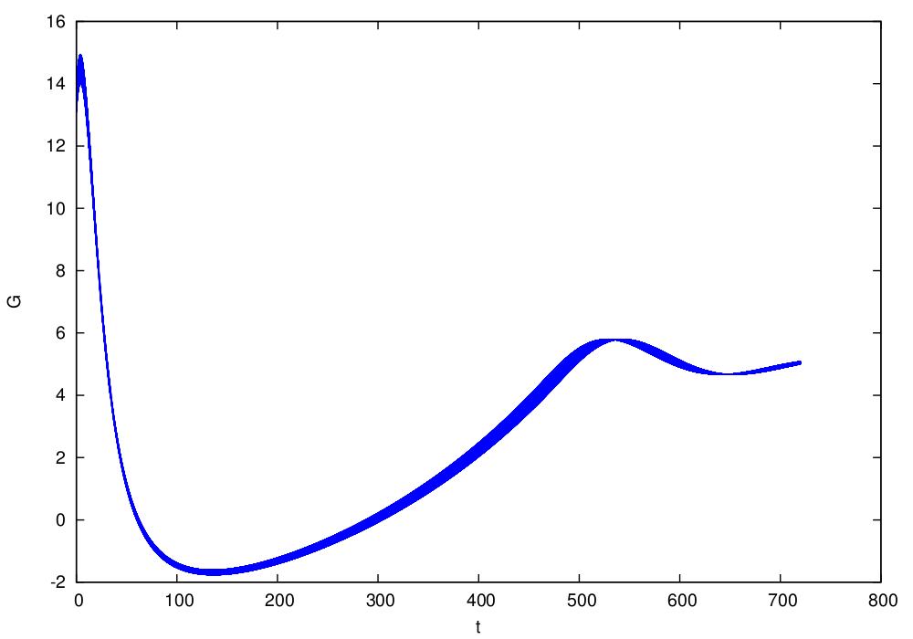
An over-approximation computed by Flow* for Strategy I is shown below. The time horizon is $[0,720]$ :

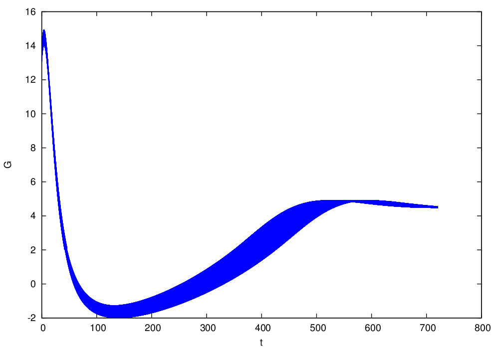
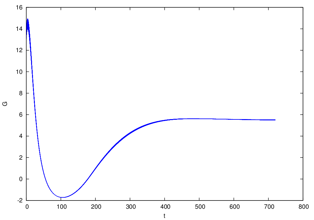
Similarly, we show the figures of the overapproximations computed by Flow* for Strategy II and Strategy III.

References

[1] R. Bergman, Y. Ider, C. Bowden, C. Cobelli. Quantitative estimation of insulin sensitivity. In The American Journal of Physiology, volume 236, pages 667-677, The American Physiological Society, 1979.

[2] R. Bergman, L. Phillips, C. Cobelli. Physiologic evaluation of factors controlling glucose tolerance in man: measurement of insulin sensitivity and $\beta$ -cell glucose sensitivity from the response to intravenous glucose. In The Journal of Clinical Investigation, volume 68, pages 1456-1467, The American Society for Clinical Investigation, 1981.

[3] R. Bergman, D. Finegood, M. Ader. Assessment of insulin sensitivity in vivo. In Endocrine Reviews, volume 6, pages 45-86, Endocrine Society, HighWire Press, 1985.

[4] M. Fisher. A semiclosed-loop algorithm for the control of blood glucose levels in diabetics. In IEEE transactions on biomedical engineering, volume 38(1), pages 57-61, IEEE,
1991.

[5] D. Chisholm, E. Kraegen, D. Bell, D. Chipps. A semiclosed loop computer-assisted insulin infusion system. In The Medical journal of Australia, volume 141, pages 784–789, Australasian Medical Publishing Company Proprietary Limited, 1984.

[6] S. Furler, E. Kraegen, R. Smallwood, D. Chisholm. Blood glucose control by intermittent loop closure in the basal mode: computer simulation studies with a diabetic model. In Diabetes Care, volume 8, pages 553–561, American Diabetes Association, 1985.