Spring pendulum | Theory of Hybrid Systems

Download

Flow*

Model description

We study the behavior of the planar spring-pendulum described in [1]. It consists of a solid ball of mass $m$ and a spring of natural length $L$ . The spring constant is $k$ .

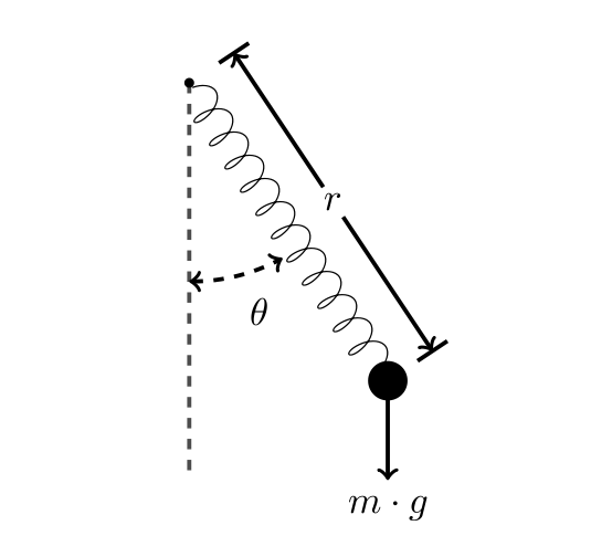
We study the evolutions of the length $r$ of the spring and the angle $\theta$ between the spring and the vertical. They are modeled by the following differential equations

$\left\{ \begin{array}{lcl} m\cdot \ddot{r} & = & m\cdot r\cdot \dot{\theta}^2 + m\cdot g \cdot \cos(\theta) - k\cdot (r - L) \\ r^2 \cdot \ddot{\theta} & = & -2\cdot r\cdot \dot{r} \cdot \dot{\theta} - g\cdot r\cdot \sin(\theta) \end{array}\right.$

which can be equivalently translated to the first-order ODE as below.

$\left\{ \begin{array}{lcl} \dot{r} & = & v_r \\ \dot{\theta} & = & v_\theta \\ \dot{v}_r & = & r\cdot v_\theta^2 + g\cdot \cos(\theta) - k\cdot (r - L) \\ \dot{v}_\theta & = & -\frac{(2\cdot v_r \cdot v_\theta + g\cdot \sin(\theta))}{r} \\ \end{array} \right.$

The constants are set as $k = 2$ , $L = 1$ , and $g = 9.8$ .

Reachability settings

We consider the initial set $r\in [1.19,1.21]$ , $\theta\in [0.49,0.51]$ , $v_r = 0$ and $v_{\theta} = 0$ .

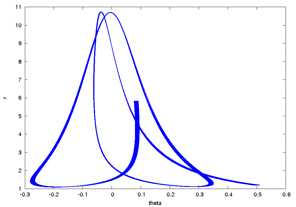
Results

The following figure shows an overapproximation computed by Flow* for the time horizon $[0,10]$ .

References

[1] J. D. Meiss. Differential Dynamical Systems (Monographs on Mathematical Modeling and Computation), Book 14, SIAM publishers, 2007.