Classification
| # of variables | # of modes | # of jumps |
|---|---|---|
| 2 | 1 | 1 |
| Type | Continuous dynamics | Guards & Invariants | Resets |
|---|---|---|---|
| hybrid | linear polynomial | linear polynomial | linear polynomial |
Download
| Flow* model I | neuron_I.model |
| Flow* model II | neuron_II.model |
Description of model I
The general dynamics of the model of spiking neurons is defined by the following ODE.
![\[ \left\{ \begin{array}{rcl} C\cdot \dot{v} & = & k\cdot (v - v_r) \cdot (v - v_t) - u + I \\ \dot{u} & = & a\cdot (b\cdot (v - v_r) - u) \end{array} \right. \]](https://ths.rwth-aachen.de/wp-content/ql-cache/quicklatex.com-c113c8189713a5dbf0419d37877ff152_l3.png "Rendered by QuickLaTeX.com")
wherein the constant parameters are given by  ,
,  ,
,  ,
,  ,
,  and
and  . The value of
  is
is  when
when  , otherwise it is
  . Whenever the value of
  reaches
  , its value is reset to
  and meanwhile
  is updated to
  .
.
Reachability settings for model I
We consider the initial set defined by ![v \in [-61,-59]](https://ths.rwth-aachen.de/wp-content/ql-cache/quicklatex.com-7831e366c72b06312f8cc15ae8e1bf1c_l3.png "Rendered by QuickLaTeX.com") ,
, ![u \in [-1,1]](https://ths.rwth-aachen.de/wp-content/ql-cache/quicklatex.com-7bc3e2193962113126bc8047d0f70549_l3.png "Rendered by QuickLaTeX.com") .
.
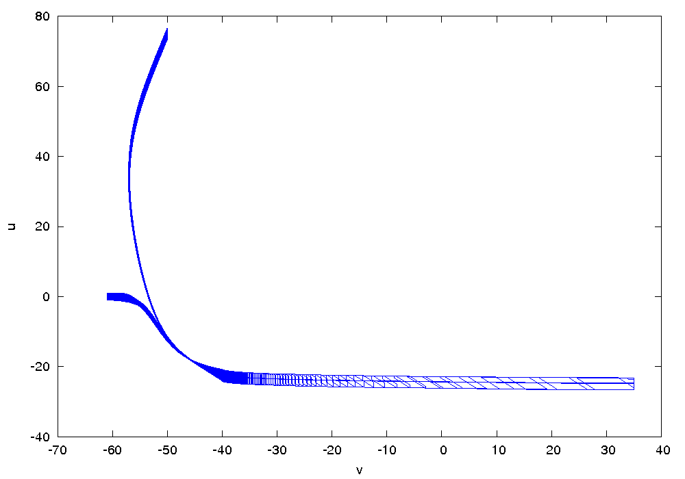
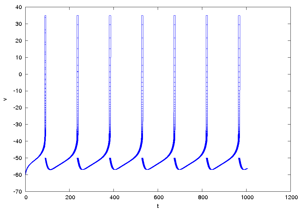
Results for model I
The following figures show an overapproximation computed by Flow* for the time horizon ![[0,1000]](https://ths.rwth-aachen.de/wp-content/ql-cache/quicklatex.com-54ec6d1712d91ddee1f9391eab56ba82_l3.png "Rendered by QuickLaTeX.com") .
.
Description of model II
As the second example, the constant parameters are given by ,  ,
,  ,
,  , ,
, ,  and
and  . The values of , are reset to
  and
and  respectively when
  .
.
Reachability settings for model II
We consider the initial set defined by ![v \in [-50.5,-49.5]](https://ths.rwth-aachen.de/wp-content/ql-cache/quicklatex.com-f98fb7e1e0b5b61ca10be335f666b480_l3.png "Rendered by QuickLaTeX.com") ,
, ![u \in [-0.5,0.5]](https://ths.rwth-aachen.de/wp-content/ql-cache/quicklatex.com-80b2eac3fdedb6121d2f7392309258b4_l3.png "Rendered by QuickLaTeX.com") .
.
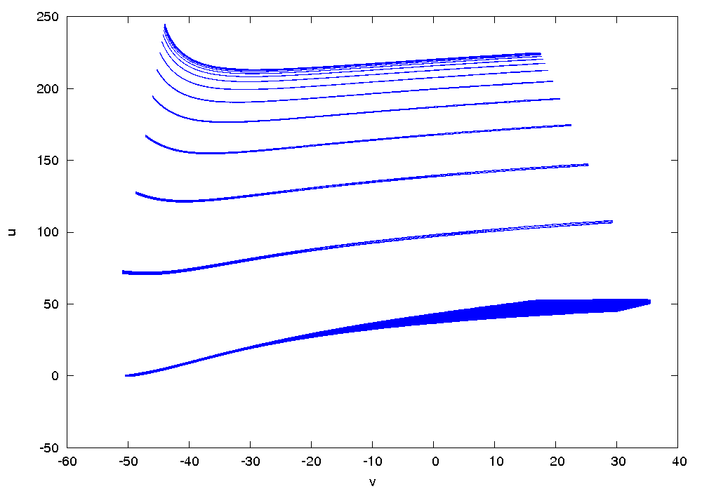
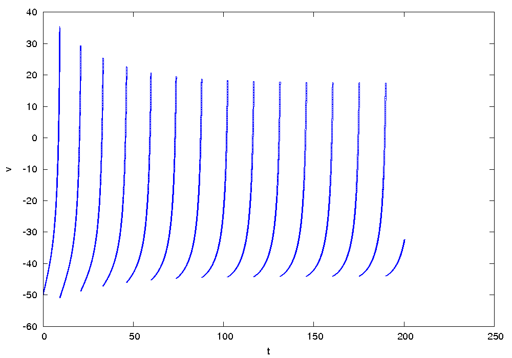
Results for model II
The following figures show an overapproximation computed by Flow* for the time horizon ![[0,200]](https://ths.rwth-aachen.de/wp-content/ql-cache/quicklatex.com-2e8f3c9781d1317852220527ac9aa4a3_l3.png "Rendered by QuickLaTeX.com") .
.