Non-holonomic integrator | Theory of Hybrid Systems

Classification

# of variables	# of modes	# of jumps
3	4	5

Type	Continuous dynamics	Guards & Invariants	Resets
hybrid	non-linear polynomial	non-linear polynomial	identity

Download

Flow*

nonholonomic.model

Model description

A simplified version of the hybrid control for Brockett’s non-holonomic integrator is described by the following ODE.

$\left\{ \begin{array}{lcl} \dot{x} & = & u \\ \dot{y} & = & v \\ \dot{z} & = & x\cdot v - y\cdot u \end{array} \right.$

wherein $u$ , $v$ are the control inputs defined by

$u \ = \ \left\{ \begin{array}{ll} 1, & x^2 + y^2 \leq |z| \\ -x + \frac{2\cdot y\cdot z}{x^2 + y^2}, & x^2 + y^2 > |z| \end{array} \right.$

$v \ = \ \left\{ \begin{array}{ll} 1, & x^2 + y^2 \leq |z| \\ -y + \frac{2\cdot x\cdot z}{x^2 + y^2}, & x^2 + y^2 > |z| \end{array} \right.$

Reachability settings

We consider the initial set $x = 0$ , $y = 0$ and $z \in [14.9,15.1]$ .

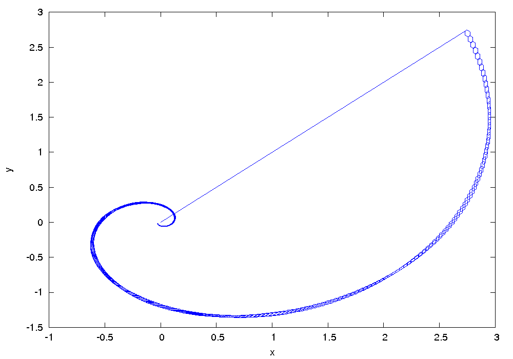
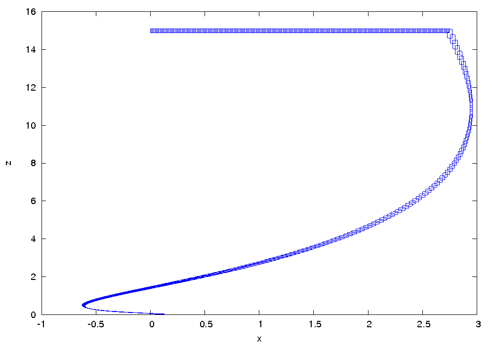
Results

The following figures show an over-approximation computed by Flow* for the time horizon $[0,7.5]$ :

References

[1] J. Hespanha, A. Morse. Stabilization of nonholonomic integrators via logic-based switching. In Automatica, volume 35(3), pages 385–393, Elsevier, 1999.