LMI-based three-vehicle platoon | Theory of Hybrid Systems

Classification

# of variables	# of modes	# of jumps
9	2	2

Type	Continuous dynamics	Guards & Invariants	Resets
hybrid	linear polynomial	half-space	constant

Download

Flow*	vehicle_platoon_3.zip
SpaceEx	3_vehicle_platoon.zip

Model description

We consider the platoon of $3$ vehicles guided by a leader illustrated in Fig.1.

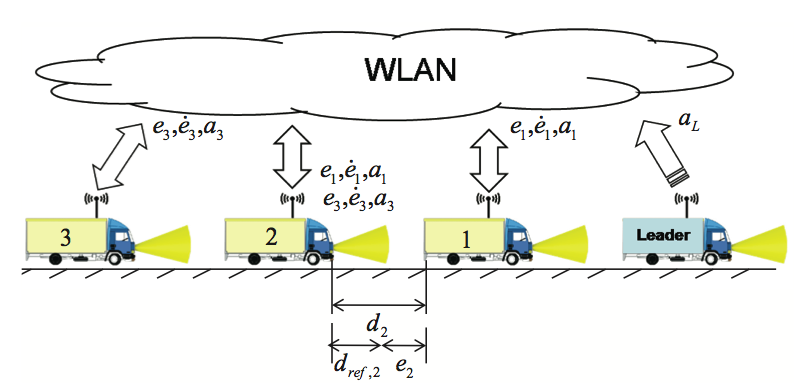
Figure 1: WLAN cooperative platoon with three vehicles and a leader ahead.

The spacing error $e_i$ is defined as the difference between the distance $d_i$ of the truck $i$ to its predecessor and a reference distance $d_{ref,i}$ .

(1) $\begin{equation*} e_i = d_i -d_{ref,i}. \end{equation*}$

The goal of the reachability analysis for this system is to determine a lower bound for $d_{ref,i}$ assuring collision-free driving.

The dynamics of the platoon is described by the following differential equation

(2) $\begin{equation*} \dot x = Ax + Ba_L, \end{equation*}$

where $A$ is a constant system matrix, $B$ is a constant input matrix and $a_L$ the acceleration of the leader considered here as an uncertain input [1,2].

The state vector is $x = [e_1, \dot{e_1}, a_1, e_2, \dot{e_2}, a_2, e_3, \dot{e_3}, a_3]$ where $a_i$ is the acceleration of vehicle $i$ .

In case of no communication problems, these matrices are given as follows

(3) $\small \begin{align*} A_c &= \left(\begin{smallmatrix} 0 & 1 & 0 & 0 & 0 & 0 & 0 & 0 & 0 \\ 0 & 0 & -1 & 0 & 0 & 0 & 0 & 0 & 0 \\ 1.6050 & 4.8680 & -3.5754 & -0.8198 & 0.4270 & -0.0450 & -0.1942 & 0.3626 & -0.0946 \\ 0 & 0 & 0 & 0 & 1 & 0 & 0 & 0 &0 \\ 0 & 0 & 1 & 0 & 0 & -1 & 0 & 0 &0 \\ 0.8718 & 3.8140 & -0.0754 & 1.1936 & 3.6258 & -3.2396 & -0.5950 & 0.1294 & -0.0796 \\ 0 & 0 & 0 & 0 & 0 & 0 & 0 & 1 & 0 \\ 0 & 0 & 0 & 0 & 0 & 1 & 0 & 0 & -1 \\ 0.7132 & 3.5730 & -0.0964 & 0.8472 & 3.2568 & -0.0876 & 1.2726 & 3.0720 & -3.1356 \end{smallmatrix}\right), \\ B_c &= \left(\begin{smallmatrix} 0 \\ 1 \\ 0 \\ 0 \\ 0 \\ 0 \\ 0 \\ 0 \ \end{smallmatrix}\right). \end{align*}$

In case of total disruption of the communication, the matrices describing the system are given by

(4) $\small \begin{align*} A_n &= \left(\begin{smallmatrix} 0& 1.0000& 0& 0& 0& 0& 0& 0& 0\\ 0& 0& -1.0000& 0& 0& 0& 0& 0& 0\\ 1.6050& 4.8680& -3.5754& 0& 0& 0& 0& 0& 0\\ 0& 0& 0& 0& 1.0000& 0& 0& 0& 0\\ 0& 0& 1.0000& 0& 0& -1.0000& 0& 0& 0\\ 0& 0& 0& 1.1936& 3.6258& -3.2396& 0& 0& 0\\ 0& 0& 0& 0& 0& 0& 0& 1.0000& 0\\ 0& 0& 0& 0& 0& 1.0000& 0& 0& -1.0000\\ 0.7132& 3.5730& -0.0964& 0.8472& 3.2568& -0.0876& 1.2726& 3.0720& -3.1356 \end{smallmatrix}\right) \\ B_n &= \left(\begin{smallmatrix} 0 \\ 1 \\ 0 \\ 0 \\ 0 \\ 0 \\ 0 \\ 0 \ \end{smallmatrix}\right). \end{align*}$

The platoon is modelled as a hybrid automaton. Its continuous dynamics constitute thereby the continuous states. The communication breakdowns, however, trigger the discrete switches from one continuous state to another. We consider the following hybrid automata describing the worst case scenario of a hazard loss of communication between all members of the platoon.

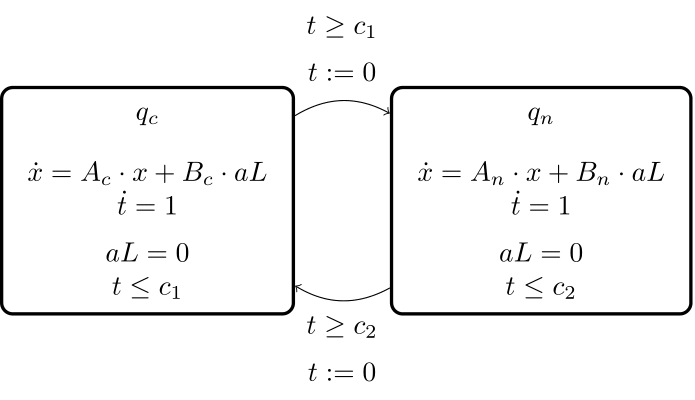
Discrete switches can be modelled as spontaneous, true or guard free transitions (Fig.2(a)) [3]. Otherwise, a clock can be added making therefore the switching dependent on time (Fig.2(b)).

Alternatively, switching can be forced if the algorithm computing the reachable set attains a fix point. That corresponds, in this context, to an invariant reachable set. Simulations during the control design help to determine the time horizon $T$ after which the controlled system reaches a stable state. For our case study, we have $T=12s$ .

In this example, the sets $D_c$ and $D_n$ corresponding respectively to the state space domains of the continuous states $q_c$ and $q_n$ are taken, for this particular application, equal to $\mathbb{R}^9$ . Otherwise the user is free to make a different but suitable choice. Furthermore, the decision on the values of the time constants $c_1$ and $c_2$ of the hybrid model in Fig.2(b) is also left to the user.

Reachability settings

The initial set is specified by

$e_i \in [0.9,1.1], i\in{1,\ldots,3}$
$\dot{e_i} \in [0.9,1.1], i\in{1,\ldots,3}$
$a_i \in [0.9,1.1], i\in{1,\ldots,3}$
$c_1,c_2 = 2$
The uncertain input for this setup was set to $a_L=0$

The initial location is $q_c$ and the time horizon is set to $T=12$ . The set of bad states are the states where $e_1 \geq 1.7$ .

Results

Results gained with SpaceEx:

References

[1] I. Ben Makhlouf, J.P. Maschuw, P. Hänsch, H. Diab, S. Kowalewskiand, D. Abel. Safety Verification of a Cooperative Vehicle Platoon with Uncertain Inputs Using Zonotopes. In Proceedings of the 18th International Federation of Automatic Control World Congress (IFAC’11), pages 9769-9774, Elsevier, 2011.

[2] I. Ben Makhlouf, H. Diab, S. Kowalewski. Safety Verification of a Controlled Cooperative Platoon Under Loss of Communication Using Zonotopes. In Proceedings of the 4th IFAC Conference on Analysis and Design of Hybrid Systems (ADHS’12), pages 333-338, Elsevier, 2012.

[3] I. Ben Makhlouf, and P. Hänsch, S. Kowalewski. Comparison of Reachability Methods for Uncertain Linear Time-Invariant Systems. In Proceedings of the European Control Conference 2013 (ECC’13), pages 1101- 1106, IEEE, 2013.

[4] J.P. Maschuw. Platoon Control and Reconfiguration Based on Linear Matrix Inequalities. In Fortschritt-Berichte VDI. Reihe 8, Mess-, Steuerungs- und Regelungstechnik, Volume 1216, VDI, 2012.

[5] J. Maschuw, D. Abel. Longitudinal vehicle guidance in networks with changing communication topology. In Proccedings of IFAC-Symposium Advances in Automotive Control (AAC’10), pages 785-790, Elsevier, 2010.

[6] J. Maschuw, G. Keler, D. Abel. LMI based control of vehicle platoons for robust longitudinal guidance. In IFAC World Congress, Volume 17, pages 12111-12116, Elsevier, 2008.