Lac operon | Theory of Hybrid Systems

Download

Flow*

Model description

The dynamics of the lac operon model presented in [1] is defined by the following ODE.

$\left\{ \begin{array}{lcl} \dot{I}_i & = & -2 \cdot k_3 \cdot I_i^2 \cdot \frac{k_8\cdot R_i\cdot G^2 + \tau}{k_3\cdot I_i^2 + \mu} + 2\cdot k_{-3} \cdot F_1 \\ & & + \frac{(k_5\cdot I_e - (k_9 + k_{-5})\cdot I_i)\cdot k_{-2}\cdot \chi \cdot k_4 \cdot \eta \cdot (k_3\cdot I_i^2 + \mu)}{k_7\cdot (k_2\cdot (k_8\cdot R_i\cdot G^2 + \tau) + k_{-2}\cdot (k_3\cdot I_i^2 + \mu))} \\ \dot{G} & = & -2\cdot k_8\cdot R_i\cdot G^2 + \frac{2\cdot k_{-8}\cdot (k_8\cdot R_i\cdot G^2 + \tau)}{k_3\cdot I_i^2 + \mu} \\ & & + \frac{k_9\cdot I_i\cdot k_{-2}\cdot \chi \cdot k_4 \cdot \eta \cdot (k_3\cdot I_i^2 + \mu)}{k_7\cdot (k_2\cdot (k_8\cdot R_i\cdot G^2 + \tau) + k_{-2}\cdot (k_3\cdot I_i^2 + \mu))} \end{array} \right.$

wherein the constants are given by

$\begin{array}{llll} k_2 = 4\cdot 10^5, & k_{-2} = 0.03, & k_3 = 0.2, & k_{-3} = 60, \\ k_4 = 1, & k_5 = 0.6, & k_{-5} = 0.006, & k_6 = 3\cdot 10^{-6}, \\ k_7 = 3\cdot 10^{-6}, & k_8 = 0.03, & k_{-8} = 1\cdot 10^{-5}, & k_9 = 5000, \\ R_i = 0.01, & \chi = 0.002002, & \eta = 0.005, & F_1 = 0.0001, \\ I_E = 91100, & \tau = 0.008. \end{array}$

Reachability settings

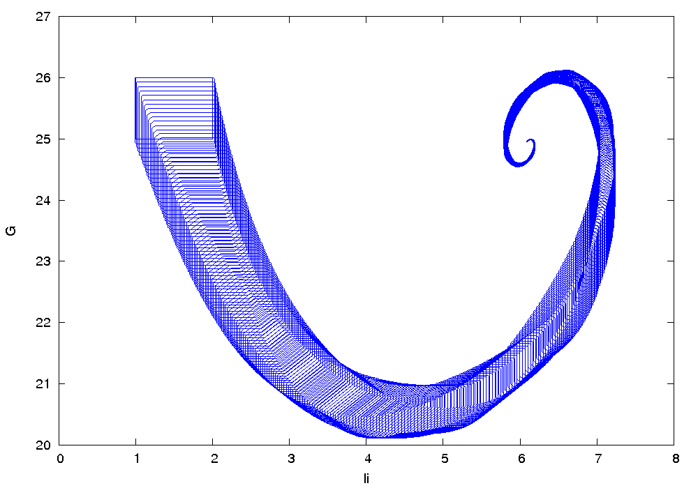
We consider the initial set $I_i\in [1,2], G\in [25,26]$ .

Results

The following figure shows an overapproximation computed by Flow* for the time horizon $[0,150]$ :

References

[1] E. Klipp, R. Herwig, A. Kowald, C. Wierling, H. Lehrach. Systems Biology in Practice: Concepts, Implementation and Application. Wiley-Blackwell, 2005.