Download
| Flow* | biology_II.model |
Model description
We present a nine-dimensional continuous model which is adapted from a biological system given in [1]. The modeling ODE is given as below.
![\[ \left\{ \begin{array}{lcl} \dot{x}_1 & = & 3 \cdot x_3 - x_1 \cdot x_6 \\ \dot{x}_2 & = & x_4 - x_2 \cdot x_6 \\ \dot{x}_3 & = & x_1 \cdot x_6 - 3 \cdot x_3 \\ \dot{x}_4 & = & x_2 \cdot x_6 - x_4 \\ \dot{x}_5 & = & 3 \cdot x_3 + 5 \cdot x_1 - x_5 \\ \dot{x}_6 & = & 5 \cdot x_5 + 3 \cdot x_3 + x_4 - x_6 \cdot (x_1 + x_2 + 2 \cdot x_8 + 1) \\ \dot{x}_7 & = & 5 \cdot x_4 + x_2 - 0.5 \cdot x_7 \\ \dot{x}_8 & = & 5 \cdot x_7 - 2 \cdot x_6 \cdot x_8 + x_9 - 0.2 \cdot x_8 \\ \dot{x}_9 & = & 2 \cdot x_6 \cdot x_8 - x_9 \end{array} \right. \]](https://ths.rwth-aachen.de/wp-content/ql-cache/quicklatex.com-c8c14774537dc3b670ea030f37ed2e5a_l3.png "Rendered by QuickLaTeX.com")
Reachability settings
We consider the initial set ![x_1,x_2,x_3,x_4,x_5,x_6,x_7,x_8,x_9\in [0.99,1.01]](https://ths.rwth-aachen.de/wp-content/ql-cache/quicklatex.com-d9e60dd20a7abd37d05a5cb91a28dc06_l3.png "Rendered by QuickLaTeX.com") .
.
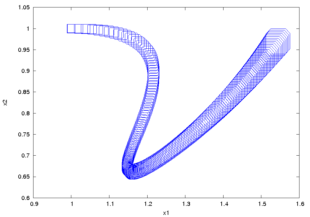
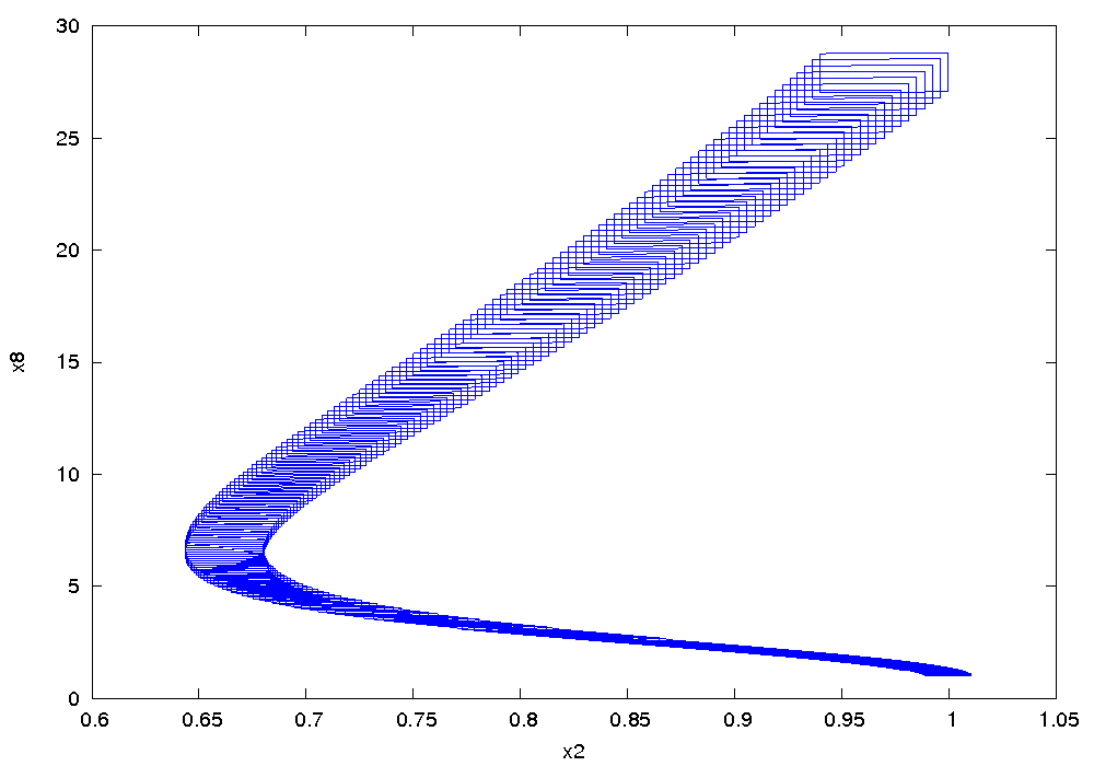
Results
The following figure shows an overapproximation computed by Flow* for the time horizon ![[0,2]](https://ths.rwth-aachen.de/wp-content/ql-cache/quicklatex.com-776f9661293135845dbde0bc8d512264_l3.png "Rendered by QuickLaTeX.com") .
.